Learn how to Use vlookup in Google Sheets

vlookup is a robust software that permits customers to seek for particular information in a big dataset. Whether or not you are a enterprise proprietor or just somebody who works with information, mastering the vlookup operate can prevent time and make it easier to make extra knowledgeable choices.

You could be a whole newbie to vlookup. Or maybe you’re extra accustomed to Excel and need to know easy methods to execute this method in Google Sheets.

Both approach, you’ll discover step-by-step directions and helpful ideas under to be sure you’re utilizing the vlookup operate appropriately and retrieving correct outcomes out of your dataset.

Desk of Contents

What does vlookup do in Google Sheets?

Vlookup is a operate in Google Sheets that searches for a particular worth within the leftmost column of a desk or vary and returns a corresponding worth from a specified column inside that vary.

The syntax for the vlookup operate is as follows:

Vlookup(search_key, vary, index, [is_sorted])

• search_key is the worth that you just need to seek for.
• vary is the desk or vary that you just need to search in.
• index is the column quantity (ranging from 1) of the worth you need to retrieve.
• is_sorted is an non-obligatory argument that signifies whether or not the info within the vary is sorted in ascending order. If this argument is about to TRUE or omitted, the operate assumes that the info is sorted and makes use of a quicker search algorithm. If this argument is about to FALSE, the operate makes use of a slower search algorithm that works for unsorted information.

For instance, when you’ve got a desk with an inventory of product names within the first column and their corresponding costs within the second column, you should utilize the vlookup operate to search for the worth of a particular product primarily based on its identify.

The Advantages of Utilizing vlookup in Google Sheets

Utilizing vlookup can prevent numerous time when looking out via giant datasets. It is an effective way to shortly discover the info you want with out having to scroll via tons of of rows manually.

Utilizing vlookup in Google Sheets additionally:

• Saves effort and time. You possibly can shortly retrieve data from giant datasets by automating the search and retrieval course of via vlookup. This may prevent numerous effort and time in comparison with manually looking for data in a desk.
• Reduces errors. When looking for data manually, there’s a threat of human error, corresponding to mistyping or misreading data. Vlookup can assist you keep away from these errors by performing correct searches primarily based on actual matches.
• Will increase accuracy. Vlookup helps make sure that you’re retrieving the right data by permitting you to seek for particular values in a desk. This can assist you keep away from retrieving incorrect or irrelevant data.
• Improves information evaluation. You possibly can analyze information extra effectively by utilizing vlookup to check and retrieve information from completely different tables. This can assist you simply determine patterns, traits, and relationships between information factors.
• Offers flexibility and customization. Vlookup permits you to specify the search standards and select which columns to retrieve information from, making it a flexible and customizable software that can be utilized for a variety of duties.

Learn how to Use vlookup in Google Sheets

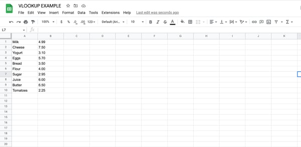
1. Open a brand new or present Google Sheet.
2. Enter the info you need to seek for in a single column of the sheet. For instance, you might need an inventory of product names in column A.
3. Enter the corresponding information you need to retrieve in one other column of the sheet. For instance, you might need an inventory of costs in column B.
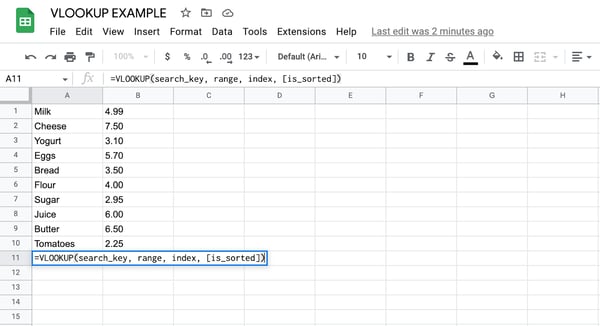
4. Determine which cell you need to use to enter the vlookup method, and click on on that cell to pick it.
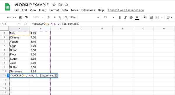
5. Sort the next method into the cell:

   =VLOOKUP(search_key, vary, index, [is_sorted])

   

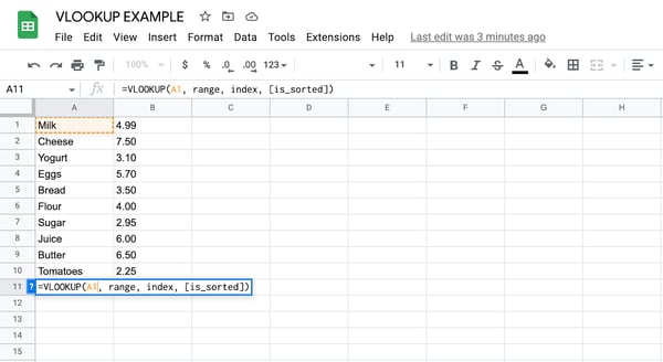
6. Change the “search_key” argument with a reference to the cell containing the worth you need to seek for. For instance, if you wish to seek for the worth of a product named “Milk” and “Milk” is in cell A1, you’d substitute “search_key” with “A1”
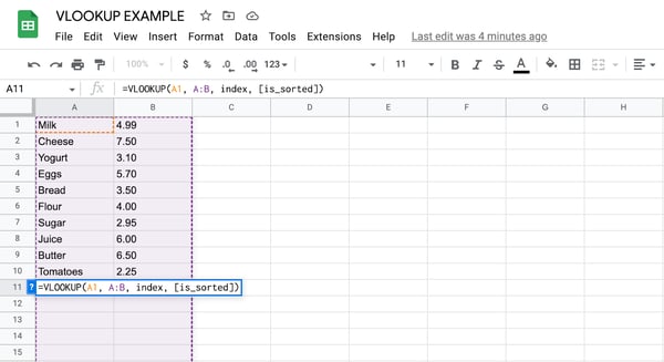
7. Change the “vary” argument with a reference to the vary of cells that incorporates the info you need to search in. 

   For instance, in case your product names are in column A and your costs are in column B, you’d substitute “vary” with “A:B”.

   You too can simply click on and drag your mouse over the vary of cells the vlookup ought to use to retrieve the info in the event you’re working with a smaller dataset.

   

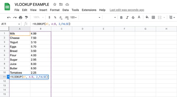
8. Change the “index” argument with the variety of the column containing the info you need to retrieve. For instance, if you wish to retrieve costs from column B, you’d substitute “index” with “2”.
9. If the info in your vary is sorted in ascending order, you may omit the ultimate “[is_sorted]” argument or set it to “TRUE”. If the info just isn’t sorted, you must set this argument to “FALSE” to make sure correct outcomes.
10. Press Enter to use the method and retrieve the specified information.

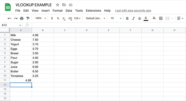
That is it! The vlookup operate ought to now retrieve the corresponding information primarily based on the search key you specified. You possibly can copy the method to different cells within the sheet to retrieve further information.

vlookup Instance

Let’s check out a sensible instance of easy methods to use the vlookup operate in Google Sheets.

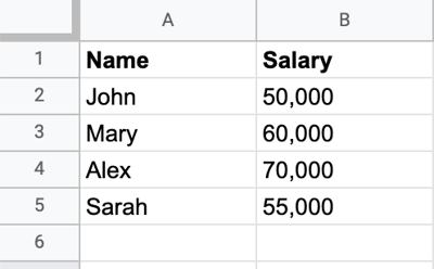
Suppose you’ve got a desk that lists the names of workers in column A and their corresponding salaries in column B. You need to search for the wage of an worker named “John” utilizing the vlookup operate.

As soon as the info is entered right into a Google Sheet, you could resolve which cell you need to use to enter the vlookup method, and click on on that cell to pick it earlier than typing within the following method:

=VLOOKUP(“John”, A:B, 2, FALSE)

The vlookup operate ought to now retrieve the wage of John, which is 50,000. Here is how the method works:

Within the first argument, “John” is the search key, which is the worth you need to search for within the leftmost column of the desk. Within the second argument, “A:B” is the vary you need to search in, which incorporates each columns A and B.

Within the third argument, “2” is the index of the column you need to retrieve information from, which is column B (since salaries are listed in column B).

The fourth argument, “FALSE”, signifies that the info within the vary just isn’t sorted in ascending order.

So the method searches for the identify “John” within the leftmost column of the desk, finds the corresponding wage in column B, and returns that worth (50,000).

Finest Practices for Utilizing vlookup

There are a number of key issues to recollect when utilizing vlookup in Google Sheets to make sure it really works correctly and returns correct information.

Ensure that the info is in the identical row.

First, be sure that the info you need to return is in the identical row as the worth you are looking for. In any other case, vlookup will not have the ability to discover it.

Type the primary column by ascending order.

Guarantee that the primary column of your information vary is sorted in ascending order.

This may make sure that the vlookup operate returns the right outcomes. If not, be sure you use the FALSE argument within the method.

Embrace headers within the vlookup method.

In case your information vary contains headers, you should definitely embody them in your vlookup method in order that the operate is aware of the place to search out the related information. In any other case, the operate might not know which column to look in and will return incorrect outcomes.

For instance, in case your columns have headers in Row 1 of the sheet corresponding to “Value,” “Title,” or “Class,” be certain these cells are included within the “vary” part of the method.

Make use of the wildcard character.

The wildcard character (*) can be utilized within the lookup worth to characterize any mixture of characters.

For instance, suppose you’ve got an inventory of product names within the first column of a knowledge vary, and also you need to search for the gross sales for a product referred to as “Chocolate Bar.”

Nonetheless, the identify of the product within the information vary is listed as “Chocolate Bar – Milk Chocolate.” On this case, an actual match lookup wouldn’t discover the gross sales for the “Chocolate Bar” product.

Right here is the way you would come with the wildcard character within the Google Sheets vlookup method:

=VLOOKUP(“Chocolate Bar*”, A2:B10, 2, FALSE)

It is necessary to notice that when utilizing a wildcard character, vlookup will return the primary match it finds within the first column of the info vary that matches the lookup worth.

If there are a number of matches, it should return the primary one it finds. Due to this fact, it is necessary to make sure that the lookup worth is particular sufficient to return the specified outcome.

Match your method to the case of the info you’re looking for.

Keep in mind that vlookup is case-sensitive, so the worth you enter into the method should match the case of the worth within the cells.

For instance, for example you’ve got a knowledge vary that features a column of product names, and the product names are listed in numerous circumstances in numerous cells, corresponding to “apple,” “Apple,” and “APPLE.”

In case you’re utilizing VLOOKUP to seek for the gross sales of a selected product, you could be sure that the lookup worth in your method matches the case of the info within the information vary.

Getting Began

The vlookup operate in Google Sheets is extraordinarily helpful in the event you’re coping with giant datasets in advanced spreadsheets. It will probably appear sophisticated to make use of at first, however with a little bit of observe, you’ll get the cling of it.

Simply bear in mind to maintain greatest practices in thoughts and, in case your vlookup isn’t working, use the guidelines above to troubleshoot.

Supply hyperlink

from Digital Marketing – My Blog https://ift.tt/OcH53gQ
via IFTTT